Field Projects
Data Collection
The quality of data collected plays a major role in establishing a genuine screening criteria result for any EOR process. The collected data might contain problems that can affect the quality of dataset, in particular, duplicate projects, missing data, inconsistent data and special cases.
The problem of duplicate and inconsistent information in the dataset was solved by referring to the SPE work published on the field projects. All the published work referred therefore, provided an authentic dataset of field projects free from inconsistent and duplicate information. The special cases were however, analyzed by studying the relationship between box-plots and cross-plots for the different parameters.
Finally, the distribution of Surfactant-Polymer flooding projects applied in different countries is shown in figure 1. It can be conferred from the figure that approximately 79% of the field projects were applied in USA.
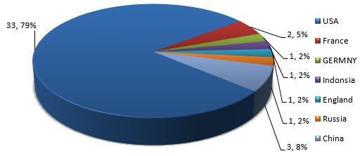
Figure 1 World surfactant-polymer flooding projects (From Oil & Gas Journal EOR surveys)
The remaining 9 field projects were applied in Germany, France, Indonesia, England, Russia and China with 3 field projects in China, 2 in France, while the remaining countries conducted 1 field project each.
Data Distribution
Figure 2 shows a histogram of reservoir temperature of the dataset. It shows that the Surfactant-polymer chemical flooding is implemented in different ranges of reservoir temperature from 65-200°F. It also shows that the minimum value of reservoir temperature at which surfactant-polymer flooding method was implemented at 65°F, while highest was at 200°F. The highest peak was observed between 65-80°F. Approximately, 71% of the temperature values lied between 70-120°F.

Figure 2 Reservoir temperature range of the dataset
Figure 3 below shows a histogram of reservoir depth for 41 surfactant-polymer chemical flooding projects. The figure shows that the peak for reservoir depth is between 1000-2000 feet. The majority of the values fall between the reservoir’s depths of 500-2000 ft, with more than 50% of the values falling in this range. Only 1 project lies between the highest value range of 7000 and 7500 ft.
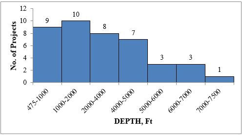
Figure 3 Reservoir depth range of the dataset
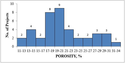
Figure 4 Porosity range of the dataset
Figure 4 shows a histogram of reservoir porosity of the dataset for 40 field projects. The highest frequency porosity lies between 17 to 23%. Approximately 52% of the porosity values lie in this range. The maximum porosity value of 34% is shown between 31-34%.
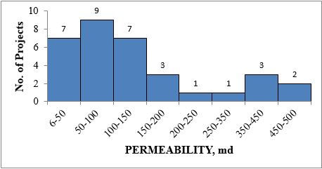
Figure 5 Reservoir permeability range of the dataset
Figure 5 shows a histogram of reservoir permeability of sandstone formations. The permeability range is across 35 field projects. 7 permeability values of reading above 1000md were excluded as special cases. These fields had high values as they consisted of unconsolidated formation. Majority of the permeability values lie in the range of 6-150md. Approximately 71% of the permeability values lie between 10-150md. The minimum value of 6md was of the reservoir in Bothamsall field of the United Kingdom.
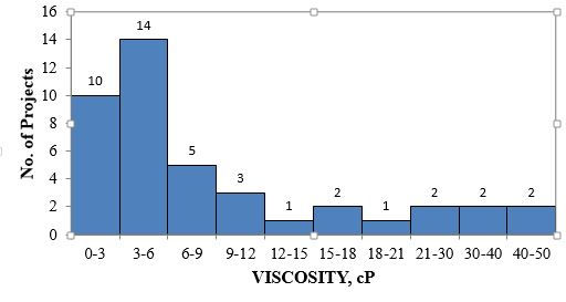
Figure 6 Oil viscosity range of the dataset
Figure 6 shows a histogram of oil viscosity of the dataset across 42 field projects. The figure is shows high frequency to the left. The highest peak is for the range of 3-6 cP. Approximately, 72% of the viscosity values are in the 0-12 cP range. Few oil viscosity values ranged from 21-50 cP, with the maximum value of 50 cP. The values of 45 and 50 cP were observed for the field projects conducted in China.
Figure 7 shows a histogram of oil gravity °API of the dataset across 39 field projects. It can be inferred from the histogram that most of the values lie in the range of 28-42°API suggesting that Surfactant-Polymer flooding projects are generally applied in reservoirs containing light oil. The distribution, as can be seen is skewed to the left. Approximately, 72% of the oil gravity values lie between the 28-41° API range.

Figure 7 Oil gravity range of the dataset
Figure 8 shows the histogram for oil saturation (start). The dataset for oil saturation (start) comprise of 35 field projects. The highest peak in the distribution lies between 30% and 35%. The diagram is skewed to the right. Also, 66% of the data values fall between 30 and 40%. This is usually the residual oil saturation at the end of water-flooding.

Figure 8 Oil saturation (start) range of the dataset
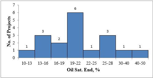
Figure 9 Oil saturation (end) distribution of the dataset
Figure 9 shows the oil saturation (end) distribution of the dataset across 16 data points ranging from 10 to 28%. The highest oil saturation (end) frequency occurs between 19 and 22%. Approximately, 69% of the oil saturation (end) values fall between 13 and 22% range.
Figure 10 shows the box-plots for different parameters for surfactant-polymer chemical flooding process. Data value ranges were provided for each parameter (minimum and maximum value) after omitting the data analyses. The minimum and maximum value range was illustrated by the distance between the opposite end of the whiskers. Additionally, the box-plots also show information such as mean and median of each parameter.

Figure 10 Left- Right-Box plots of Reservoir temperature, Depth, Oil viscosity, Oil gravity, Reservoir porosity & permeability, Brine Salinity & Hardness, Oil saturation start & end
Summarization of Field Dataset
Table below gives the range for surfactant-polymer flooding on the basis of statistical analysis for a cleaned dataset. The summary includes all the parameters which eventually decide success or failure of a surfactant-polymer flooding project. The statistical parameters used to define the range were mean, median, standard deviation, minimum and maximum values.
The ranges for the parameters was eventually compared with the previous work and the differences were noted.
- The concluded summary of oil gravity had a range from 17°API to 45°API. Brasear (1978), Carcaoana (1982) and Goodlett (1986) suggested a value greater than 25°API, while Taber (1997) suggested a value to be greater than 20°API. Aldasani and Bai gave a range of 22°API to 39°API, with and average value of 34.8°API.
- Oil viscosity in the study has a range of 0.32cP to 50cP, while authors like Caracoana (1982), Peter H. (2984) and Goodlett (1986) suggested a value less than 30cP. On the other hand, Taber (1997) suggested a value of less than 35cP for oil viscosity. Aldasani and Bai concluded a range of 15.6 to 3 cP and a mean of 9.3cP.
- Temperature range in the study was from 65°F to 200°F. Most of the authors suggested the value to be less than 200°F (Table 2.3), while Caracoana (1982) and Al-Bahar (2004) suggested a value less than 180°F and 158°F respectively. The temperature range differed from previous work conducted by Aldasani and Bai, as they concluded a range of 122-155°F with a mean of 138.5°F
- Depth range was concluded to be between 475 ft to 7500ft which differed from the values of less than 7000ft and 9000ft suggested by Caracoana (1982) and Goodlett (1986) respectively.
- Porosity value ranged from 11 to 34% in the study. However, Brashear (1978), Caracoana (1982) and Goodlett (1986) suggested a value of greater than 20%.
- Permeability range was concluded to be between 6md and 500md. This range differed from the value proposed by most of the authors. Brashear (1978), Caracoana (1982), Peter H. (1984), Goodlett (1986), Taber (1997) and Al-Bahar (2004) suggested a value greater than 20md, 35md, 40md, 40md, 40md and 50md respectively.
LABORATORY DATA
Most of the screening criteria work which has been published so far consists of field projects and pilot projects for various EOR processes. However, continuous laboratory research is been carried out to improve EOR processes. A good amount of research is also carried out in Surfactant-polymer chemical flooding process.
A dataset of laboratory work was established comprising of experiments for Surfactant-polymer flooding method. The dataset source comprised of information obtained from various publications in the SPE literature of onepetro. The dataset includes different experiments published to study properties and efficiency of surfactant-polymer flooding. All the injection experiments were carried out in various cores to study the efficiency of the flood for oil recovery.
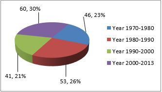
Figure 11 Laboratory surfactant-polymer flooding experiments from 1970-2013
Figure 11 shows the distribution of laboratory work on surfactant-polymer flooding carried out over the years. It shows the number of experiments which were conducted from 1970-2013. The turn of 20th century saw the most number of experiments carried out to check the efficiency of SP flooding. Sixty experiments in our dataset were executed in the years 2000 to 2013. Also, 99 experiments took place from 1970 to 1990, which is EOR boom period.
Figure 12 shows the different surfactants which were used in the experiments to establish a surfactant slug. Including the 4 basic surfactants such as Anionic, Non-ionic, Cationic, and Zwitterionic surfactants, there emerged a class of Bio-surfactants, which are generated through microbes and bacteria. The pie-chart (figure 3.22), illustrates the percentage and number of experiments conducted in each category. Zwitterionic dataset was the smallest as this class of surfactants was only recently proposed for research.

Figure 12 Distribution of types of Surfactants used in laboratory dataset
Conventional, anionic surfactants were used in most of the experiments, resulting in the biggest dataset. Over 79% of 200 experiments used anionic surfactants to study their effect on oil recovery.
Figure 13 depicts the type of polymers used in the dataset. It shows the percentage and number of 4 different types of polymer viz. Hydrolyzed polyacrylamide, xanthan gum, bio-polymer and associating polymer used in the experiments. HPAM was the most common polymer used; while only a few experiments were conducted using a new emerging class of Associating polymer.
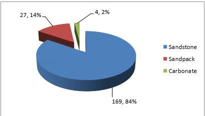
Figure 13 Types of Cores used in the Laboratory dataset
Sandstone cores, sandpacks and carbonate cores were the 3 major types of cores used in the tests. More than 80% of the tests were conducted in the sandstone cores including Berea, Bentheimer, Briarhill and Reservoir cores. Few tests (14%) were conducted in sandpacks, while even fewer were conducted in non-fractured carbonate cores.
Figure 14 shows a cross-plot of oil viscosity vs. oil gravity of the crude oil used in different tests. One test, as is evident by the diagram showed oil viscosity of 376 cP and gravity of 16.5°F. A test using such heavy oil was conducted to study the efficiency of the surfactant-polymer flooding process in heavy oil reservoirs of Canada.

Figure 14 Cross plot of Oil viscosity vs. oil gravity
It shows a very few data-points as some experiments used crude oil with same oil viscosity and oil gravity. Also, many experiments only mentioned the oil viscosity and not the oil gravity °API.
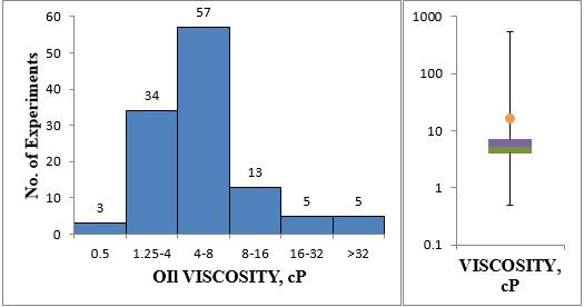
Figure 15 Oil viscosity histogram (left) and oil viscosity box-plot (right)
Figure 15 depicts the histogram and box-plot of oil viscosity values used in the experiments. The lowest oil viscosity value was of 0.5cP while the highest oil viscosity value was of 550cP, which is denoted by the >32 bar in the histogram. It can be inferred from such high oil viscosities that the surfactant-polymer flooding is being tested for recovery efficiency of heavy crude oil, to increase the application range of the method.

Figure 16 Oil Gravity histogram (left) and oil gravity box-plot (right)
Figure 16 shows the range of oil gravity °API with the help of histogram and the box-plot. The minimum value was 14.5° API and further the low values observed were between the values of 14.5 to 20°API. Such low values were observed for the experiments in which heavy crude oil with high viscosity were used. The new proposed class of zwitterionic (amphoteric) surfactants was tested for recovery in heavy oil reservoirs. A few experiments were conducted for a crude oil with viscosity of 75cP. An Alkoxy Carboxylate surfactant with large hydrophobic tail was used to check its stability in the presence of high viscosity oil. Oil recovery results for these experiments showed promising results.
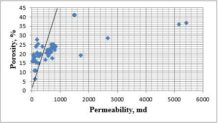
Figure 17 Cross-plot of core permeability vs. core porosity
Figure 17 shows a cross-plot of core permeability vs. core porosity. The data-points show a consistent relationship between the porosity and permeability values. However, five peremeability values lie on the higher side, over 1000md. These high permeability values were observed for sandpacks. Sandpacks are the loosely packed grains of sand which are generally used to observe the behaviour of the chemical slug in the formation and its interaction when it comes in contact with the crude oil. The minimum value observed in the cross-plot was of 106 md of reservoir core.

Figure 18 Core porosity histogram (above) and core porosity box-plot (below)
Figure 18 represents the range of core porosity with the help of a histogram and a boxplot. As we study the diagram, it can be inferred that the highest peak of core porosities was observed in the range of 18 to 22. Approximately, 76 percent of the porosity values lie between 14-26%. The lowest value of porosity observed was of 6.47%. This value was the porosity value measured for a reservoir core. The porosity box-plot shows a spread of porosity values between 6.47 to 41%, with the mean at 23.9%.

Figure 19 permeability histogram (above) and permeability box-plot (below)
Figure 19 shows the distribution of permeability values for the different cores used in the tests. It can be concluded from the histogram and permeability box-plot that the permeability values are spread over a wide range from 9.8md to over 5000md. Majority of the values in the dataset lie between 70 and 800. However, the permeability values vary significantly from one core to other core, for instance, one of the reservoir core permeability was 2668md, while most of the reservoir cores had permeability values of less than 1000md. Also, the high permeability values (greater than 1000md) are observed for sandpacks and few Bentheimer cores.
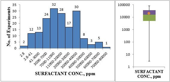
Figure 20 Surfactant slug concentration histogram (left) and box-plot (right)
Figure 20 gives the range for surfactant slug concentration used in the tests in our dataset. Majority of the values lie in the range of 5000 to 40,000 parts per million (ppm). Approximately 77% of the 175 surfactant concentration values lie in the aforementioned range. It can also be inferred that a few values are as low as 2.8ppm. Concentrations of bio-surfactants used in a few experiments had a range of 2.8ppm to 41ppm. The box-plot of surfactant slug concentration shows a mean of 20,355.6ppm. High concentration of surfactant slug (over 50,000ppm) in the subset was observed for tests which used surfactant blend of petroleum sulfonate and non-ionic surfactant. The concentration measured was a combination of these surfactants.

Figure 21 Surfactant slug size histogram (left) and box-plot (right)
Figure 21 depicts the range of surfactant slug size in terms of pore volume injected. The surfactant slug size of the subset ranged from 0.03 to 3. As can be inferred from the plots, majority of the values lie between 0.041 and 0.9. The surfactant slug size over 1PV were used in bio-surfactant tests.
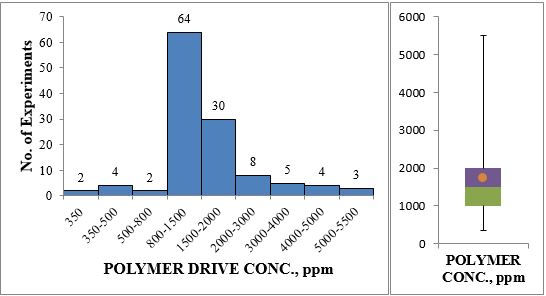
Figure 22 Polymer drive concentration histogram (left) and box-plot right
Figure 22 illustrates the range of polymer drive concentration (parts per million) with the help of a histogram and box plot. Majority of the tests were conducted with polymer concentration of 800 to 2000 ppm. 74 of the 121 values in the subset lie in this range. Few values in the dataset were high in the range of 4000-5000ppm. These were bio-polymer concentrations.
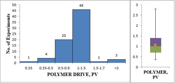
Figure 23 Polymer drive slug size histogram (left) and box-plot (right)
Figure 23 gives the range of polymer drive slug size in terms of total pore volume injected. The minimum value observed in the dataset was 0.35 PV while the maximum value observed was 2.8 PV. Majority of the values in this subset were in the range of 0.5PV to 1.5 PV. The maximum slug size of 2.8 PV was observed for a test conducted in reservoir sandstone core to achieve a favourable mobility ratio.

Figure 24 IFT between oil-water-surfactant system histogram (left) and box-plot (right)
Figure 24 shows the interfacial tension (IFT) values between oil-surfactant-water system. It can be inferred that the IFT values in the dataset had a wide spread from 0.0001 dynes/cm to 4.2 dynes/cm. The higher IFT values were observed for the oil-surfactant-water system in which bio-surfactants were used. Also, as can be interpreted from the IFT box-plot, the mean of the subset 0.274 dynes/cm because of these high values ranging from 1 dynes/cm to 4.2 dynes/cm.
Figure 25 shows the range of dynamic adsorption of anioinic surfactants on sandstone adsorbent. The adsorption was measured in terms of milligrams of surfactant adsorbed per gram of adsorbent. Majority of the adsorption values ranged from 0.1mg/g to 0.6mg/g. Few of the surfactants had high surfactant adsorption, ranging from 1 mg/g to 4.2 mg/g. These were observed for reservoir sandstone cores, where adsorption increases due to reservoir heterogenity.
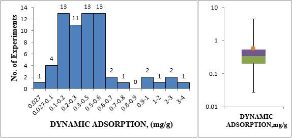
Figure 55 Dynamic adsorption histogram (left) and box-plot (right)
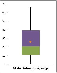
Figure 56 Static adsorption box-plot
Figure 26 shows the range of static adsorption of anionic surfactants on kaolinite adsorbent. It can be inferred from the box-plot that the adsorption ranges from 0.4 mg/g to as high as 66.1 mg/g. When compared with dynamic adsorption, static adsorption has higher values. This can be attributed to kaolinite adsorbent used in the static adsorption experiments. Since clay has higher surface area than sandstone, more surfactant is adsorbed on it.
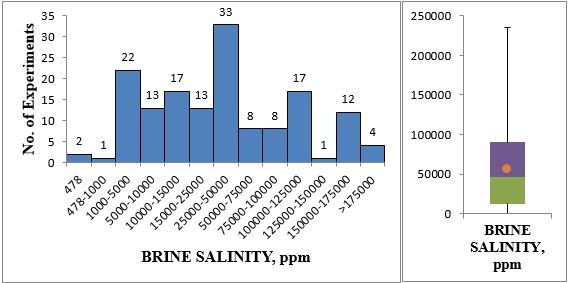
Figure 27 Brine salinity histogram (right) and box-plot (left)
Figure 27 shows the brine salinity distribution with the help of a histogram and a box-plot. It can be inferred from the graph that the minimum and maximum values for brine salinity was 478ppm and 235,000ppm respectively. Such high brine salinity values were observed for surfactants which were tested for harsh reservoir conditions of salinity and hardness.
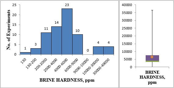
Figure 28 Brine hardness histogram (right) and box plot (left)
Figure 28 illustrates the distribution of brine hardness subset. It can be inferred that the brine hardness values had a wide spread from 130ppm to as high as 40,000ppm. The high hardness values were observed in some tests conducted to check surfactant stability in harsher reservoir conditions conataining hard brines.
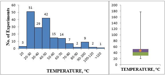
Figure 29 Temperature histogram (left) and box plot (right)
Figure 29 shows the range of temperatures under which the experiments were conducted. The values show a wide range of spread between 20°C to 177°C. It can be inferred from the figure that few experiments were conducted under high temperatures for instance; one test was conducted at a temperature of 177°C (350°F) to test the stability of surfactant (akyl aryl sulfonate) at such high temperature.
Figure 30 illustrates a cross plot of Surfactant slug concentration (parts per million) vs. the tertiary oil recovery of fraction of oil in place after waterflooding for all the tests performed. The oil recovery, as can be concluded varies significantly from core to core. This prominent difference between oil recoveries for the cores can be attributed to the type of cores being used to check the efficiency of the surfactant-polymer flooding. Berea sandstone cores, Briarhill sandstone cores, Bentheimer sandstone cores were used in most of the tests. These standard cores are more homogenous than the reservoir cores.

Figure 30 Cross-plot of surfactant concentration vs. tertiary oil recovery (after waterflooding)
Low residual oil recovery in the reservoir cores was attributed to the heterogeneity of the rock, which affected the stability of the chemical slug which resulted in higher surfactant retention (adsorption) and affected the micro-emulsion phase, which in turn affected the size of the oil bank formed. Surfactant slug concentration injected in the cores also affected the tertiary oil recovery. For example, in tests where low concentration of bio-surfactants was used, the oil recovery was poor. However, when high concentration of surfactants (47,600 ppm) was injected in a core, all of the residual oil was recovered as indicated by the cross-plot above. Figure 61 shows the range of percentage of tertiary oil recovery after waterflooding. The values of the subset had a wide spread between 19.5% to 100% tertiary oil recovery. Most of the low oil recoveries were observed for reservoir sandstone cores, while higher tertiary oil recoveries were measured for more homogenous Berea sandstones, Briarhill sandstones.

Figure 31 Tertiary oil recovery histogram (right) and box-plot (left)
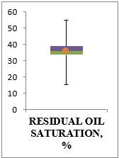
Figure 32 Residual oil saturation box-plot